

Creating land cover maps to monitor the most important variable of global change
|
- By Dale Wilson and Björn Schröder, University of the
Witwatersrand
Land cover is a fundamental variable that impacts on and links many parts of the human and physical environments. Land cover change is thus regarded as the single most important variable of global change.
Our knowledge of land cover dynamics is poor however, mainly due to the accuracy of land cover data [1]. In this light, the monitoring of vegetation in Southern Africa via satellite data has become increasingly important. This is because it is increasingly linked to variation in agricultural production and climate change, with serious resultant implications for wildlife management and tourism [2]. Remote sensing imagery in combination with geographic information systems (GIS) software can be used in the application of land cover monitoring.
Land cover classification using remote sensing has become an important tool for creating land cover maps for areas all around the world. “The production of thematic maps, such as those depicting land cover, using an image classification is one of the most common applications of remote sensing”[1]. These types of maps are essential in answering the questions associated with land cover change and land use change to the physical environment.
“Land use denotes the human employment of the land and is studied largely by social scientists. Land cover denotes the physical and biotic character of the land surface and is studied largely by natural scientists” [3]. Land cover map comparisons are the most common analysis technique used in remote sensing. This is done through the comparison of two land cover maps of the same region from different years. The difference in land use/ cover change identified within the region can be used to address the issues as to why these areas are changing.
This article outlines the creation of a land cover map, from the initial fieldwork through to the classification procedure done in the geographic information systems lab using Landsat TM data.
Study area
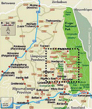
The area in which the study took place is in the Lowveld region near Acornhoek and Hoedspruit situated in the south of the Limpopo Province. The area has a high concentration of game farms and is in close proximity to the Kruger National Park (see Fig 1).
Large parts of this region were part of the Kruger National Park prior to 1923. After 1923, some parts of the Kruger National Park were returned and employed for various land uses such as cattle farming and commercial farming.
Since then, these farms have either continued in use or have been changed back into natural game areas [5]. This area is an ideal area for a land cover classification map since it boasts an area with different land cover types, from natural vegetation to farming, as well as different stages of regeneration.
This area also has large communities of people and it may be possible to view the impacts that these communities have on the surrounding land use and land cover types.
Methodology
The methodology of creating the land cover map was split up into two parts - fieldwork and lab classification. Fieldwork was undertaken from 1 to 5 April 2007 at the Wits Rural Facility near Acornhoek in the Limpopo Province. In order to identify and geo-reference land cover types for the region in study, fieldwork was required. The equipment used consisted of a global positioning system (GPS), notebook and a camera.
The fieldwork required going out into the field and identifying all the different land cover types for the area. Once a land cover point or ‘training site’ was chosen, a GPS point was taken while standing in the centre of this land cover type.
Detailed notes and a photo of these areas were taken so that classification in the lab went smoothly. Five different areas were chosen to study and for training site collection (Table 1).
| Site | GPS Co-ordinates | Number of training sites |
| Wits Rural Facility | 24° 33’ 09” S 31° 05’ 49” E |
14 |
| Acornhoek | 24° 35’ 43” S 31° 03’ 44” E |
13 |
| Royal Malewane | 24° 31’ 08” S 31° 09’ 43” E |
14 |
| Plantations | 24° 35’ 09” S 30° 58’ 20” E |
8 |
| Welverdiend | 24° 34’ 45” S 31° 21’ 34” E |
9 |
Table 1: Chosen study areas
A total of 58 training sites were taken and included many different land cover types. These land cover types ranged from open spaces and savanna to urban areas and plantations. Once the land cover training sites had been obtained and their relative GPS co-ordinates stored on the GPS unit, classification could commence back at the University of the Witwatersrand GIS Lab, using Idrisi Kilimanjaro software.
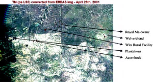
Prior to the fieldwork being done, the Landsat 2008_February_Article for the area had been obtained. These 2008_February_Article were dated to April 2001 and were taken using the Landsat TM satellite.
The first step was transferring the GPS co-ordinates from the GPS onto a text file in an XYZ format where X denotes the South GPS co-ordinate; Y denotes the East co-ordinate and Z, the relative reference raining site.
Many GPS systems these days have a direct cable from the GPS to the computer that creates the text file automatically. In this case, it was done manually. Once the text file had been created and is in the correct format, it was possible to import this file into Idrisi Kilimanjaro. Using the general conversion tool, IXZIDRIS, the text file was converted into a vector file and listed the various training site points on a blank map, using the generic lat/long co-ordinate system.
A common problem with this technique arose due to the fact that the text file had to be in a specific format with specific reference to the number of spaces after the Z component. There should be only one space after the Z component and the next point should be on the next line.
Now that the training sites were geographically represented on a blank map as a vector file, it was possible to overlay the points onto a map of the area. Bands 1, 2 and 3 of the Landsat TM 2008_February_Article were displayed with their blue, green and red components respectively to create a full colour image. The vector file was then overlaid to give a map indicating the points in relation to the ground (Fig 2).
Two methods of classification were used for the creation of the land cover map, supervised and unsupervised classification.
Unsupervised classification
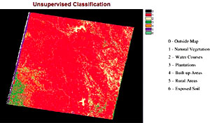
In unsupervised classification, the dominant spectral response patterns that occur within an image are extracted [5]. Using the module Cluster and setting a maximum number of eight clusters using the broad generalisation, an unsupervised map was created. The number of clusters was set to eight after using the module Histo and identifying that there were eight main clusters, after which the spectral responses were too small. Using the module Assign, the clusters outside of the given map area were given the number 0.
In the final map using the unsupervised classification, six land cover types were created (see Fig 3).
According to Eastman [5] “no classification is complete without an accuracy sssessment”. Accuracy assessment was implemented firstly by checking that the specific clusters coincide with the photos and notes taken for the sites during the fieldwork. The next step was classifying the six clusters into land cover types that reflect the relative clusters colours.
Supervised classification
Supervised classification according to Eastman [5] is where “the user develops the spectral signatures of known categories, such as urban and forest, and then the software assigns each pixel in the image to the cover type to which its signature is most similar”. “Supervised classification is the procedure most often used for quantitative analyses of remote sensing image data” [6].
Due to the fact that the training sites had already been established and were already in vector format for use in Idrisi, it was possible to create the signature file for classification. Before running the Makesig module, the training sites had to be digitised into polygon format so that the Makesig module had the correct number of pixels per cluster so that an accurate classification could occur.
From the unsupervised classification process, it was found that there were approximately eight to ten strong spectral responses that would give a satisfactory Makesig output. After a study of the 58 training sites and with notes being taken, it was accepted that eight broad land cover types were chosen and these were then digitised over the 58 training site vectors. It was then possible to run the Makesig module.
The Makesig module creates a signature file for each land cover type making it possible to classify the various pixels on the map. A common error came about from the Makesig module and was identified as not having a large enough digitised area for each training site.
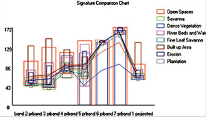
Once the Makesig module had finished, SigComp was run using the signature files made in Makesig. SigComp creates a graph which displays the land cover types and their relative reflectance values across each band used in the creation of the signature files. From the graph it was possible to identify the signature with the highest reflectance values across the entire bands (Fig 4). This would suggest which signature group was the most dominant in the map.
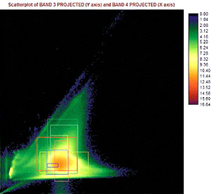
It was suggested that the module Scatter also be used to compare the signatures of the land cover types. The image created plots of the pixels of two bands, where the reflectance of each forms the axis [4].
Fig 5 shows the scatterplot of Bands 3 and 4 with an overlay of the characteristics of each signature. The image suggests that although the signatures are very close together, they are still distinguishable and it is possible to use the supervised classification hard classifiers in Idrisi. The graph and Scatterplot suggested that classification, using hard classifiers in Idrisi would be possible.
The first classification module attempted was that of Mindist. This module is a minimum distance to means classifier and “calculates the distance of a pixel’s reflectance values to the spectral mean of each signature file, and then assigns the pixel to the category with the closest mean” [4].
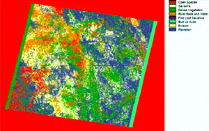
Mindist was first run using the raw distance and infinite search distance. The resulting map did not output well and showed signatures that were mixed and did not agree with the initial land cover training sites. Mindist was run again, but used the normalised distance. The resulting image displayed (see Fig 6) was better, but while some land cover types were accurate, others were not.
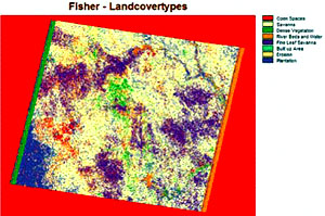
The last hard classifier used was Fisher. This module uses linear discriminant analysis to analyse the signatures and create the land cover maps [5]. The Fisher module was run, and produced the most successful land cover map (see Fig 7).
Results
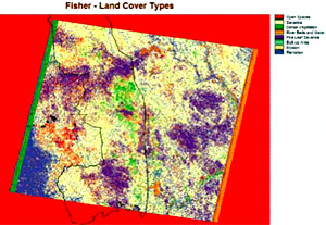
Comparison between the fieldwork notes and the various land cover maps created using the modules in Idrisi meant that it was possible to identify which map reflected the best land cover types for the region. The map created using Fisher reflected this and as such will be used as the final land cover map for the study area.
Figure 8 shows the final map with an overlay of the borders of the Kruger National Park and the training sites from the fieldwork. From the map it is evident to see that the most dominant land cover type for the region is savanna. This is the dominant land cover type for the Lowveld/ Bushveld region. The next most dominant land cover type is the fine leafed savanna, followed by the dense vegetation and then plantations.
The other land cover types such as urban areas, open areas, erosion, and rivers are small in cover but still come up well on the map. The overlay of the Kruger National Park is useful in analysing the accuracy of the map due to the fact that if the Kruger Park area showed that it was mainly water or urban areas we would know that this was false and could not use the map. The Kruger Park comes up well on this map and is dominated by the savanna, fine leaf savanna and dense vegetation. This is coherent with the land cover types observed when visiting the Kruger Park and surrounding areas.
The final land cover map is successful in portraying most of the dominant land cover types for the region. There are a few signatures such as erosion and river beds and water that create some inconsistencies on the final map. This will be discussed further on.
Discussion
The final land cover classification methods used were both that of unsupervised and supervised classification. Although the unsupervised classification did not create a satisfactory land cover map for the area, it did, however give the number of clusters with the highest reflectance value and as such, the number of land-cover types to be used in the supervised classification process. A recurring problem in many of the maps created was that certain land cover types were shown in areas where it is known that there is another dominant land cover type.
Foody [1] refers to this as thematic accuracy, “which is the correspondence between the class label assigned by the classification and that observed in reality”. An example of this is in the Pipedminmax map where the dominant land form is plantations. This cannot be true because we know that the Kruger National Park is composed of natural vegetation and not commercial plantations.
According to Eastman [5], this could be the case due to overlapping signatures “because of the inadequate nature of the definition of land cover classes”. Most land cover types were correctly defined, except for the erosion signature. In retrospect, it would have been better to have classified the erosion cluster as ‘exposed soil’. Exposed soil and erosion would theoretically show similar signatures [7].
Tanser & Palmer [8] suggest that GPS and geo-referencing errors contribute to the signature overlapping errors. This is due to the fact that accuracy of the GPS used could have resulted in some training sites having similar signatures to others. This would explain the occurrence of some land cover types in other areas, such as dense vegetation in dams.
According to Palmer and Van Rooyen [9], the output 2008_February_Article are also highly influenced by the type of data used. The data used in the creation of these maps were from Landsat TM satellite and dated to April 2001. Since 2001, there have obviously been changes to the land cover of the area. There has been urban growth, removal of plantations, land regeneration as well as variability in the rainfall which affects the vegetation in the region.
All these changes indicate that the study region could have been very different in 2001 and could affect the training sites that were chosen in the first place. The unavailability of a recent Landsat TM image for the region meant that a comparison between landcover maps was not possible and the overall accuracy of the map was reduced. Even though the Landsat TM image was relatively old, the land cover and land use of the region would not have changed so much that the land cover map would be unusable.
Limitations
In remote sensing image data interpretation, there are two main categories of error. The first category is due to labelling inconsistencies, which regards how representative training data is classified (due to mixed pixels or class overlap). The second type of error is the classification-induced error. This can be reduced by using carefully defined classes and class numbers, classification schemes, and the choice of the feature (control point) vector [10].
It is thus very important that the training area contains as little mixed pixels as possible. They arise especially at object borders where two different objects are neighboured to each other. For this reason a buffer is computed around the object border which has a width of four pixels they say [11].
On that note, the overall accuracy is logically viewed as a problem of misclassification, where a pixel is said to be misclassified if it’s true class (as determined by ground check), is one thing but it has been assigned by the classifier as something else [12].
Finally, in terms of the Maxlike failure, it is said that the Maximum Likelihood algorithm suffers from the drawback that it typically yields noisy segmentations, where in nature larger areas of the same land cover are more likely. This effect is mainly caused by considerable noise in the input data, as a result of reflectance from neighbouring pixels.
In addition, mixed pixels composed of more than one land cover class also contribute to this effect, as they often cannot be classified uniquely [13]. However, in contrast it is said that a properly designed classifier such as the Maxlike, nearly always provides better performance, and is much less sensitive to many unmanageable factors such as atmospheric conditions [14].
Conclusion
The creation of land cover maps is an exercise characterised by many problems and challenges. These problems are caused by the data used, signatures obtained and in this case, the software used. Although these problems were time consuming, they were helpful in understanding the intricate nature of remote sensing and accuracy assessment.
For this study, both supervised and unsupervised classification methods were used and land cover maps were produced. The unsupervised classification produced a successful image but was not accurate in defining types of vegetation. The signatures that were picked up were mostly vegetation, water courses and plantations.
With the supervised classification method, various supervised techniques were used. The linear discriminant analysis classifier or Fisher produced the best output. Land cover maps are an important tool for graphically understanding changes to land cover and land use for many regions. A general consensus amongst scholars is that accuracy assessment of the land cover maps needs to be improved [1].
References
[1] G Foody: Status of land cover classification accuracy assessment, Remote Sensing of Environment: Vol. 80, pp.185– 201, 2001.
[2] CAD Sannier, JC Taylor, W Du Plessis and Campbell: Real-time vegetation monitoring with NOAA-AVHRR in Southern Africa for wildlife management and food security assessment, International Journal of Remote Sensing, Vol. 19 (4), pp. 621- 639, 1998.
[3] W. Meyer, B Turner II: Human Population Growth and Global Land-Use/Cover Change, Annual Review of Ecology and Systematics, Vol 23, pp. 39-61, 1992.
[4] http://www.suedafrika.net/maps/ mpumalimpomap3.gif, Park under Pressure, 21 May 2007.
[5] J Eastman: IDRISI Kilimanjaro Tutorial, Clark Labs, Clark University, 2003.
[6] J Richards and J Xiuping: Remote Sensing Digital Image Analysis: An Introduction, Springer, Germany, 2006.
[7] A Diouf and E Lambin: Monitoring land-cover changes in semi-arid regions: remote sensing data and field observations in the Ferlo, Senegal, Journal of Arid Environments, Vol. 48, pp129-148, 2001.
[8] F Tanser and A Palmer: Vegetation Mapping of the Great Fish River Basin, South Africa: Integrating Spatial and Multi-Spectral Remote Sensing Techniques, Applied Vegetation Science, Vol. 3:2, pp.197-203, 2000.
[9] A Palmer and A Van Rooyen,: Detecting vegetation change in the southern Kalahari using Landsat TM data, Journal of Arid Environments, Vol. 39, pp143-153, 1988.
[10] PC Smits: Multiple Classifier Systems for Supervised Remote Sensing Image Classification Based on Dynamic Classifier Selection. IEEE Transactions on Geosciences and Remote Sensing, Vol. 40 (4), pp. 801-813, 2002.
[11] D Fritsch, M Englisch, and M Sester: Automatic Classification of Remote Sensing data for GIS database revision. IAPRS, Vol. 32 (4), pp 641-648 ISPRS Commission IV Symposium on GIS –Between Visions and Applications, Stuttgart., 1998.
[12] MF Goodchild: Integrating GIS and Remote Sensing for Vegetation Analysis and Modeling: Methodological Issues. Journal of Vegetation Science, Vol. 5 (5), pp.615-626, 1994.
[13] J Keuchel, S Naumann, M Heiler, and A Siegmund: Automatic land cover analysis for Tenerife by supervised classification using remotely sensed data. Remote Sensing of Environment, Vol. 86, pp. 530–541, 2003.
[14] B Jeon and DA Landgrebe: Partially Supervised Classification Using Weighted Unsupervised Clustering. IEEE Transactions on Geosciences and Remote Sensing, Vol. 37 (2), pp. 1073-1079, 1999.
Acknowledgements
A special thank you must be given to the Wits Rural Facility, the Royal Malewane Lodge, the community of Welverdiend and the SAEON Ndlovu Node for access to their properties and hospitality during the field work. Special thanks should also be given to Dr Emma Archer for supervising this report.
Contact Dale Wilson, Wits University, Tel 083 626-8240, smudgedale@gmail.com
Article courtesy of Position IT